All machine learning algorithms rely more or less on the process of maximizing or minimizing the objective function. We often refer to a minimized function as a loss function, which is mainly used to measure the predictive power of the model. In the process of finding the minimum value, our most common method is the gradient descent method, which is very similar to the process of descending from the top of the mountain to the bottom of the valley.
Although the loss function describes the superiority and inferiority of the model, it provides us with the optimization direction, but there is no universally accurate loss function. The choice of loss function depends on the number of parameters, outliers, machine learning algorithms, the efficiency of gradient descent, the ease of derivative finding, and the confidence of prediction. This article will introduce a variety of different loss functions and help us understand the advantages and disadvantages of each function and the scope of application.
Because of the different tasks of machine learning, the loss function is generally divided into two categories: classification and regression. The regression predicts a numerical result and the classification gives a label. This article focuses on the analysis of the regression loss function.
1. Mean square error, square loss - L2 loss
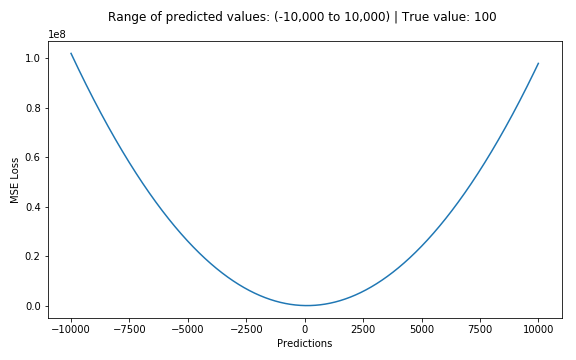
The mean squared error (MSE) is the most common error in the regression loss function. It is the sum of squared differences between the predicted and the target values. The formula is as follows:

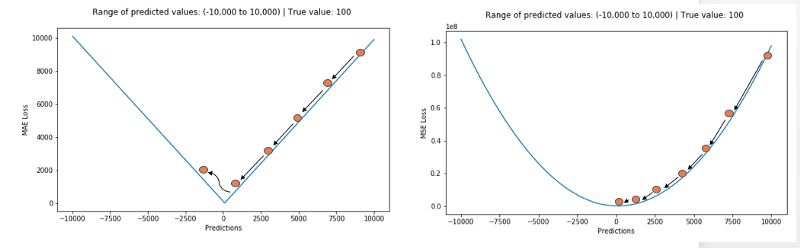
The following figure shows the curve distribution of the RMS error value, where the minimum value is the position where the predicted value is the target value. We can see that the loss function increases more rapidly as the error increases.
2. The average absolute error - L1 loss function
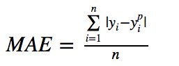
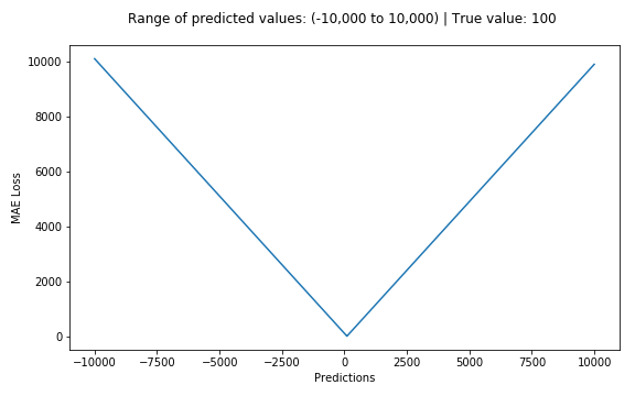
The average absolute error (MAE) is also a commonly used regression loss function. It is the sum of the absolute value of the difference between the target value and the predicted value. It represents the average error magnitude of the predicted value without considering the direction of the error. The error MBE is the error of the considered direction and is the sum of the residuals. The formula is as follows:
Comparison of average absolute error and mean square error (L1 & L2)
In general, using the mean squared error is easier to solve, but the squared absolute error is more robust to the extra-local point. Let us analyze the two loss functions in detail.
Regardless of which machine learning model, the goal is to find the point that minimizes the objective function. At the minimum, each loss function will get the minimum value. But which is the better indicator? Let's take a look at a specific example. The figure below is a comparison of the root-mean-squared error and the mean absolute error (where the purpose of the root-mean-squared error is to unite with the average absolute error):
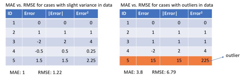
In the left graph, the predicted value is close to the target value, the error and variance are small, and the error in the right graph due to the presence of an out-of-plane point makes the error large.
Since the loss of the mean square error (MSE) at the larger error point is much greater than the mean absolute error (MAE), it will give more weight to the outliers and the model will strive to reduce the errors caused by the outliers, thus making The overall performance of the model declined.
So when the training data contains more outliers, the average absolute error (MAE) is more effective. When we process all the observations, if we use MSE for optimization we will get the mean of all observations, and using MAE we can get the median of all observations. Compared to the mean, the median is more robust to outliers, which means that the average absolute error has better robustness than the mean squared error for the outliers.
However, there is also a problem in MAE, especially for neural networks, its gradient will have a big jump at the extreme point, and a very small loss value will also cause a long time error, which is not conducive to the learning process. . In order to solve this problem, it is necessary to dynamically reduce the learning rate in solving the extreme points. MSE has good characteristics at extreme points and can converge at a fixed learning rate in time. The gradient of the MSE decreases with decreasing loss function, which makes it possible to obtain more accurate results during the final training.
In the actual training process, the MSE is a better choice if the out- side points are very important for the actual business, and the MAE will bring better results if the out-of-office points are most likely to be dead pixels. . (Note: L1 and L2 are generally the same in nature as MAE and MSE)
Conclusion: The L1 loss is more robust to the extra-oral point, but its derivative discontinuity makes the process of finding the optimal solution inefficient; the L2 loss is sensitive to the extra-oral point, but is more stable and accurate in the optimization process.
However, there are still two problems that are difficult to deal with. For example, 90% of the data in a task meets the target value of 150, while the remaining 10% of the data is between 0-30. Then the MAE-optimized model will get the predicted value of 150 while ignoring the remaining 10% (clinching towards the median value); for the MSE, because of the large losses incurred by the extra-site, it will make the model tend to In the 0-30 direction value. Both of these results are undesirable in real business scenarios.
then what should we do?
Let's take a look at other loss functions!
3. Huber loss - smooth average absolute error
Huber loss is insensitive to outliers compared to square loss, but it also maintains differentiability. It is based on absolute error but becomes square error when the error is small. We can use the hyperparameter δ to adjust this error threshold. It degenerates to MAE when δ tends to 0, and degenerates to MSE when δ tends to infinity. Its expression is as follows, which is a continuous differentiable segmentation function:
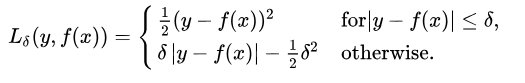
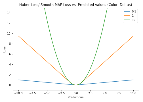
For Huber losses, the choice of δ is very important, and it determines the behavior of the model dealing with out-of-office points. Loss of L1 is used when the residual is greater than δ, and a more appropriate L2 loss is used when it is small.
The Huber loss function overcomes the shortcomings of MAE and MSE. Not only can the loss function have a continuous derivative, but also the MSE gradient can be used to obtain a more accurate minimum with the error reduction characteristics, and it is also better for outliers. Awesome.
But the good performance of the Huber loss function benefits from the well-trained hyperparameter δ.
4.Log-Cosh loss function
The logarithmic hyperbolic cosine is a loss function that is smoother than L2 and uses the hyperbolic cosine to calculate the prediction error:
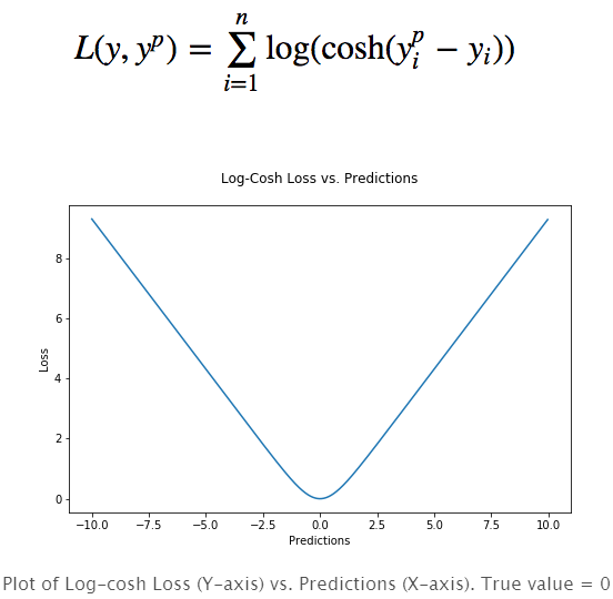
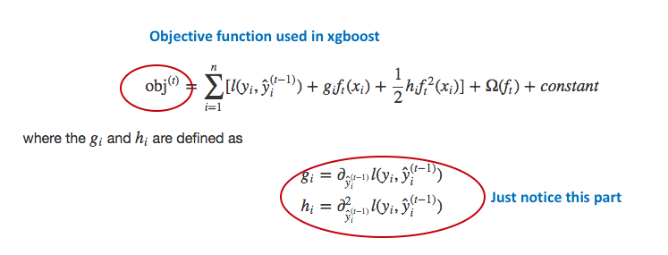
The advantage is that log (cosh(x)) is very similar to (x**2)/2 for very small errors and very close to abs(x)-log2 for very large errors. This means that the logcosh loss function can have the advantage of MSE without being affected too much by the outside point. It has all of Huber's advantages and is twice-guided at every point. Quadratic derivation is necessary in many machine learning models, such as using the Newtonian XGBoost optimization model (Hessian matrix).
But the Log-cosh loss is not perfect, it will still become constant with gradients and hessian.
5. Quantile Loss
In most real-world prediction problems, we often want to get the uncertainty of our forecast results. By predicting a range of values ​​rather than a specific value point is crucial to the decision in a specific business process.
The quantile loss function is a particularly useful tool when we need to determine the range of values ​​for the outcome. Normally we use the least square regression to predict the value interval based on the assumption that the variance of the residual value is a constant. However, many times it is not satisfied with the linear model. At this time, the quantile loss function and quantile regression are needed to save the regression model. It is very sensitive to the range of predictions and maintains good performance even with non-uniformly distributed residuals. Let's use two examples to look at the regression performance of quantile losses under heteroscedastic data.

The above figure shows two different data distributions. The left figure shows the case where the residual variance is a constant, and the right figure shows the variation of the residual variance. We use normal least squares to estimate the above two cases, where the orange line is the result of modeling. However, we can't get the interval range of the value. At this time, we need the quantile loss function to provide.

The upper and lower two dashed lines in the above chart are based on the quantile loss of 0.05 and 0.95. From the figure, you can clearly see the range of predicted value of the model after modeling. The goal of quantile regression is to estimate the conditional quantile of a given predictor. In fact, the quantile regression is an extension of the mean absolute error (when the quantile is the 50th percentile, the value is the average absolute error)
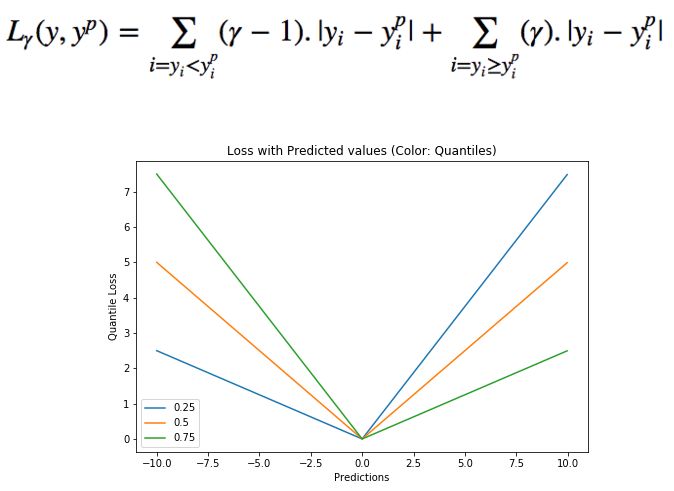
The quantile is worth choosing because we want to make positive or negative errors more valuable. The loss function will impose different penalties on the overfit and underfit based on the quantile γ. For example, selecting γ = 0.25 means that more overfitting will be punished while keeping the prediction value slightly smaller than the median value. The value of γ is usually between 0-1. In the figure, the loss function under different quantiles is described. It can be clearly seen that the positive and negative errors are unbalanced.
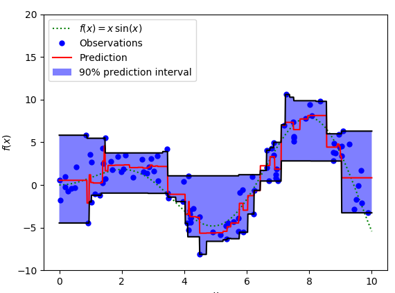
We can use the quantile loss function to calculate the interval of the neural network or tree model. The following figure is calculated based on the gradient lift tree regression value interval. The upper and lower boundaries of the 90% predicted value are calculated using the gamma values ​​of 0.95 and 0.05, respectively.
At the end of the article, we used sinc(x) simulated data to compare the performance of different loss functions. Gaussian noise and impulsive noise are added to the original data (in order to describe robustness). The following figure shows the results obtained by the GBM returner using different loss functions, where the ABCD plots are the results of the MSE, MAE, Huber, and Quantile loss functions, respectively:
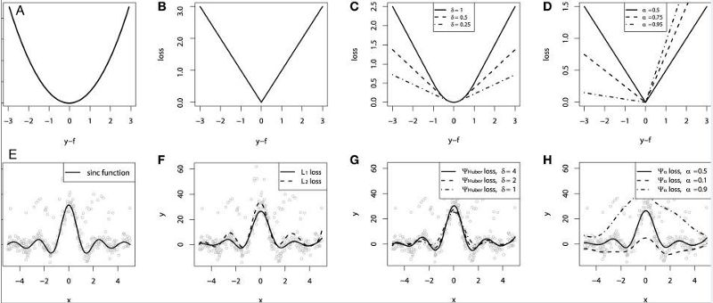
We can see that the predicted value of the MAE loss function is less affected by the impact noise, while the MSE has a certain bias; the Huber loss function is insensitive to the selection of hyperparameters, and the quantile loss is given in the corresponding confidence interval A good estimate.
It is hoped that small partners can understand the loss function in more depth from this article and choose the right function in the future work to complete the task faster and better.
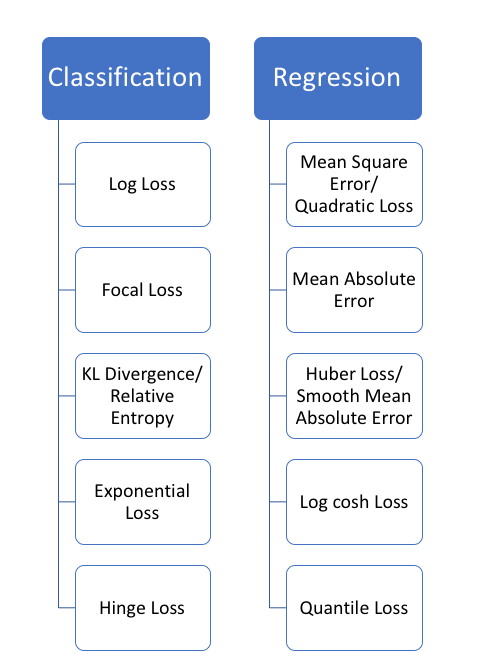
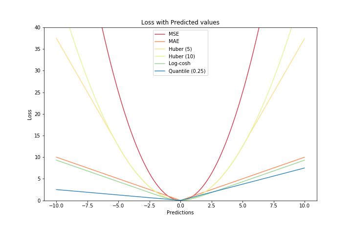
Finally, attach a diagram of some of the loss functions in this article.
Components of automobile parts
The basic unit of each part of the transportation vehicle, also called auto parts, referred to as auto parts, mainly consists of the following major parts:
Engine fittings
Throttle body, engine, powertrain, oil pump, nozzle, tensioning wheel, cylinder block, bearing bush, water pump, fuel injection, gasket, camshaft, valve, crankshaft, connecting rod assembly, piston, belt, muffler, carburetor, fuel tank, water tank, fan, oil seal, radiator, filter, generator, starter
Driveline fittings
Transmission, the gear shift lever assembly, reducer, clutch, pneumatic, electric tools, magnetic materials,, clutch disc, clutch cover, universal joint, universal ball, universal ball, the ball cage, clutch plate, transfer, scoop, synchronizer, synchronizer ring, synchronous belt, differential, differential shell, differential plate Angle gear, planetary gear, wheel frame, flange, gear box, medium Intershaft, gear, stop lever fork, drive shaft assembly, drive shaft flange
Brake fittings
Brake shoe, brake pad, brake disc, brake drum, compressor, brake assembly, brake pedal assembly, brake master cylinder, brake wheel cylinder, ABS ECU controller, electric hydraulic pump, brake camshaft, brake wheel, brake tellurium pin, brake slack adjusters, brake chamber, vacuum booster, hand brake assembly, parking brake assembly, parking brake lever assembly
Steering gear fittings
Kingpin steering knuckle ball pin...
Traveling fittings
Rear axle, air suspension system, counterweight, steel plate, tire, leaf spring, half axle, shock absorber, ring assembly, half axle bolt, axle housing, frame assembly, wheel stand, front axle
Electrical instrumentation accessories
Sensors, automotive lighting, buzzer, spark plug, battery, wiring harness, relay, audio, alarm, regulator, distributor, starter (motor), directional, automotive instrument, switch, fuse, glass lifter, generator, ignition coil, igniter
Automobile lamps and lanterns
Decorative light, headlight, searchlight, ceiling light, fog light, instrument light, brake light, taillight, turn signal, emergency light
Car modification
Tire pump, car roof frame, car top box, electric winch, car buffer, sunroof, sound insulation material, bumper, fixed wing, fender, exhaust pipe, fuel saver
Security guard against theft
Steering wheel lock, wheel lock, alarm, rearview mirror, rearview system, camera, seat belt, drive recorder, central lock,GPS, ABS, reversing radar, shift lock
The car interior
Car carpet (mat) steering wheel cover steering wheel power ball curtain, sun file...
Automotive exteriors
On the wheel hub cover, paint strip sticker license plate rack...
Comprehensive accessories
Adhesive, sealant, car tools, car spring plastic parts...
Av appliances
Tire pressure monitoring system decoder display car intercom...
Chemical nursing
Coolant, brake fluid, antifreeze, lubricating oil...
Body and accessories
Windshield wipers, car glass seat belts, airbags, instrument benches...
Maintenance equipment
Sheet metal equipment purification system tire removal machine calibration instrument...
Electric tools
Electric shear hot air gun electric jack
Auto Parts,Investment Casting Pipe,Casting For Stainless Steel,Stainless Steel Exhaust Pipes
Tianhui Machine Co.,Ltd , https://www.thcastings.com