Machine Learning: Introduction to Random Gradient Descent and Batch Gradient Descent Algorithm

Stochastic Gradient Descent

Batch Gradient Descent

Gradient descent (GD) is a widely used optimization algorithm for minimizing the loss or risk function in machine learning. Two popular variants of GD are Stochastic Gradient Descent (SGD) and Batch Gradient Descent (BGD). In this article, I’ll explain both methods from both mathematical and practical perspectives. If you find any errors, feel free to correct me!

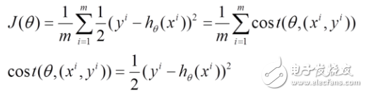
Let’s define some basic terms: h(x) represents the model we’re trying to fit, J(θ) is the loss function, θ refers to the parameters that we’re solving for iteratively, and m is the number of training samples. The goal is to find the optimal θ that minimizes the loss function.

1. Batch Gradient Descent

(1) First, compute the gradient of the loss function J(θ) with respect to each parameter θ:

(2) Then, update each parameter θ in the direction opposite to the gradient, which helps minimize the loss function:

(3) One key point here is that BGD computes the gradient using all the training examples at once, which guarantees convergence to the global minimum if the loss function is convex. However, when the dataset is large, this approach can be computationally expensive and slow. This leads us to the next method: Stochastic Gradient Descent.

2. Stochastic Gradient Descent

(1) The loss function can also be expressed as the sum of individual losses over each sample. BGD uses all samples, while SGD updates parameters one sample at a time:

(2) For each sample, we compute the partial derivative of the loss function with respect to θ and update the parameters accordingly:

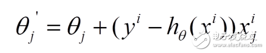
(3) Unlike BGD, SGD processes one example at a time, making it much faster for large datasets. However, this introduces more noise into the updates, so the path to the minimum isn’t as smooth. Despite this, SGD often converges quickly and can reach a solution close to the global minimum, even if not exactly perfect.

3. Which Method Gives a Better Solution for Linear Regression?

(1) Batch Gradient Descent aims to minimize the total loss across all samples, leading to the global optimal solution. It guarantees that the final parameters will give the lowest possible loss.

(2) Stochastic Gradient Descent, on the other hand, minimizes the loss per sample. While each step may not directly move toward the global minimum, the overall trend is still towards the optimal solution. Therefore, SGD usually gives a near-optimal result, especially when the data is large.

4. Global vs. Local Optima

For problems like linear regression, where the loss function is convex, GD will always converge to the global minimum. However, for non-convex problems with multiple local minima, GD might get stuck in a suboptimal solution. That’s why techniques like momentum or adaptive learning rates are often used to improve convergence.

5. Implementation Differences Between SGD and BGD

In practice, the difference between SGD and BGD lies in how they process the data. BGD computes gradients using the entire dataset, while SGD updates parameters after processing each sample. This makes SGD more suitable for large-scale machine learning tasks. In my previous blog post, I demonstrated an NMF implementation and showed how these two approaches differ. Writing code in Python would make this clearer—so I encourage you to try implementing them yourself!

[Java] view plain

// Stochastic Gradient Descent: Update Parameters

HSD LVDS Automotive High Frequency Connectors

Hsd Lvds Automotive High Frequency Connectors,Automotive High Frequency Connectors,12Pin Male Connecor For Cable,High Speed Connector For Cable

Dongguan Zhuoyuexin Automotive Electronics Co.,Ltd , https://www.zyx-fakra.com