Machine Learning: Introduction to Random Gradient Descent and Batch Gradient Descent Algorithm

Stochastic Gradient Descent

Batch Gradient Descent

Gradient descent (GD) is one of the most commonly used optimization techniques in machine learning for minimizing loss functions and risk functions. Two popular variants of GD are Stochastic Gradient Descent (SGD) and Batch Gradient Descent (BGD). This article will explore both methods from both a mathematical and implementation perspective, aiming to clarify their differences and use cases. If there are any errors, please feel free to point them out.

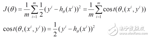
In this context, h(x) represents the hypothesis function we aim to fit, J(θ) is the loss function, θ denotes the parameters that need to be optimized iteratively, and m refers to the number of training samples. Each parameter j corresponds to a specific feature or weight in the model.

1. The Approach of Batch Gradient Descent:

(1) First, we compute the gradient of the loss function J(θ) with respect to each parameter θ. This gives us the direction of steepest ascent, which we then use to update the parameters in the opposite direction for minimization.

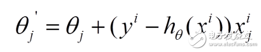
(2) Next, we update each parameter θ by moving in the negative direction of its corresponding gradient. This ensures that we are heading toward the minimum of the loss function.

(3) One key characteristic of BGD is that it computes the gradient using the entire training dataset at each iteration. While this guarantees convergence to the global minimum (in convex problems), it can be computationally expensive when the dataset is large. This limitation motivates the development of Stochastic Gradient Descent.

2. The Approach of Stochastic Gradient Descent:

(1) Unlike BGD, SGD updates the parameters using only a single training sample at a time. The overall loss function can be viewed as the average of individual sample losses.

(2) For each sample, we calculate the partial derivative of the loss function with respect to θ, and then update the parameters accordingly. This makes the process much faster per iteration, especially for large datasets.

(3) However, because SGD uses only one sample at a time, the updates are noisier compared to BGD. This means that the path taken to reach the minimum may not be perfectly aligned with the true global minimum. Despite this, over time, the algorithm tends to converge close to the optimal solution.

3. Which Method Provides the Optimal Solution in Linear Regression?

(1) Batch Gradient Descent computes the gradient using all samples, ensuring that the final result is the global minimum, assuming the problem is convex.

(2) Stochastic Gradient Descent, on the other hand, updates parameters based on individual samples. Although the updates may not always move directly toward the global minimum, the overall trend still leads to a solution that is very close to the optimal one.

4. When Does Gradient Descent Find a Global Minimum vs. a Local Minimum?

In linear regression, the loss function is typically convex, meaning there's only one minimum. Thus, gradient descent will eventually find the global optimum. However, in non-convex problems (such as those found in neural networks), there may be multiple local minima, and the algorithm might get stuck in one of them depending on the initial conditions and learning rate.

5. Implementation Differences Between SGD and BGD

When implementing these algorithms, the main difference lies in how the gradients are computed. BGD processes the entire dataset at once, while SGD processes one sample at a time. This has significant implications for performance and memory usage. For example, in Python, you can implement BGD with vectorized operations, but for SGD, you would loop through each sample individually.

[Java] view plain

// Stochastic Gradient Descent, updating parameters

FAKRA Automotive High Frequency Connectors

Fakra Automotive High Frequency Connectors,Multi-Port Rf Connectors,Fpc Automotive Connector,Automotive Terminals Connector

Dongguan Zhuoyuexin Automotive Electronics Co.,Ltd , https://www.zyx-fakra.com